
RF indicates the electromagnetic frequency that can be radiation to space, the frequency range from 300KHz to 30GHz, referred to as RF. RF is the radio frequency current, it is the abbreviation of high frequency alternating current change electromagnetic wave. Low-frequency current is the alternating current that changes less than 1000 times per second, high-frequency current is greater than 10000 times, and RF is such a high-frequency current.
Section 1 Power-related Concepts
Peak power, average power, and peak-to-average ratio PAR of the signal
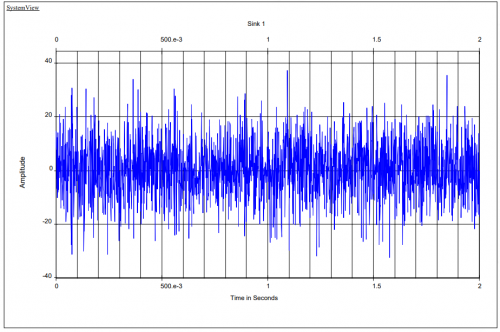
Explanation: Many signals observed from the time domain are not constant envelopes. Instead, they are as shown in the graph below. The peak power is the transient power of a shoulder peak that occurs with some probability. Usually, the probability is taken as 0.01%.
Peak power, average power, and peak-to-average ratio PAR of the signal
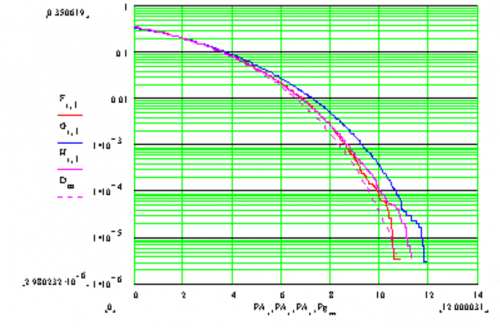
Explanation: The average power is the actual power output by the system. The peak-to-average ratio at a certain probability is the ratio of the peak power to the average power at a certain probability. For example, [email protected]%, the peak-to-average ratio under various probabilities forms a CCDF curve (complementary cumulative distribution function). The PAR at a probability of 0.01% is generally referred to as the CREST factor.
Section 2 Noise-related Concepts
Noise Definition
Noise is the interference signal encountered during signal processing that cannot exactly predict. (various types of point frequency interference do not count as noise). Common noises are from external astronomical noise, car ignition noise, thermal noise from inside the system, scattered particle noise generated by transistors and so on during operation, intermodulation products of signal and noise, etc.
Phase Noise
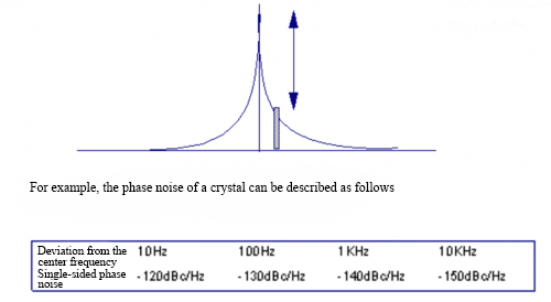
Phase noise is an indicator to measure the spectral purity of a monophonic signal such as the local oscillation. In the time domain, it is a jitter of the signal over the zero point. Ideally, a single-tone signal should be a pulse in the frequency domain. The actual single tone always has a certain spectral width, as shown below.
In general, the local oscillation signal can be considered as a random process to phase the monophonic process. Therefore, the signal has a sideband signal called phase noise. Phase noise in the frequency domain can be described quantitatively as follows: how many Hz away from the center frequency, the power per unit bandwidth compared to the total signal power.
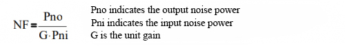
Noise Factor
The noise factor is a measure of the ability of RF components to handle small signals. It is usually defined as follows: cell input signal-to-noise ratio divided by output signal-to-noise ratio, as follows.
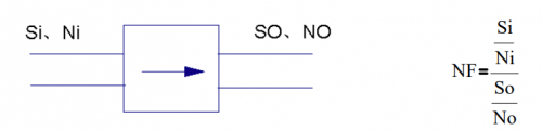
For linear units, no signal-noise intermodulation products and signal distortion are generated.
The noise factor at this point can be expressed by the following equation.
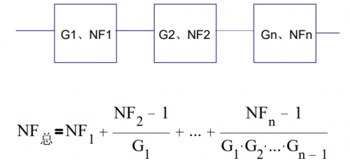
Noise factor equation for cascade networks.
Section 3 Linearity-related Concepts
The signal will have a certain degree of distortion when passing through the RF channel (here the so-called RF channel refers to the RF transceiver channel, excluding the space segment fading channel). Distortion can be divided into linear distortion and nonlinear distortion.
The main linear distortion is generated by some filters and other passive devices. Non-linear distortion is mainly generated by some amplifiers, mixers, and other active devices. In addition, the RF channel will also have some additive noise and multiplicative noise introduction.
Linear Distortion
Linear distortion can be further divided into linear amplitude distortion and linear phase distortion. These distortions can easily represent from the frequency domain, as follows.

Nonlinear Distortion
Nonlinear distortion is similar to linear distortion and can be divided into nonlinear amplitude distortion and nonlinear phase distortion. The graphical representation is as follows.
Nonlinear Amplitude Distortion
Nonlinear amplitude distortion is commonly measured by 1dB compression point, third-order cross-tuning, and third-order cutoff point. These three metrics are discussed separately below.
1dB Compression Point
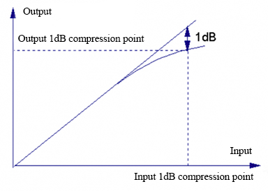
For example, in an RF amplifier, when the input signal is small, its output and input can guarantee the line relationship, the input level increases by 1dB, the output increases by 1dB accordingly, and the gain remains unchanged.
As the input signal level increases, the input level increases by 1dB, and the output will increase by less than 1dB. The gain starts to compress, the input signal level when the gain is compressed by 1dB is called the input 1dB compression point at which the output signal level is called the output 1dB compression point. As shown.
Third-order Intermodulation
Third-order intermodulation (two-tone third-order intermodulation) is an important indicator used to measure nonlinearity, and the amplifier is still used here as an example to illustrate the third-order intermodulation indicator.
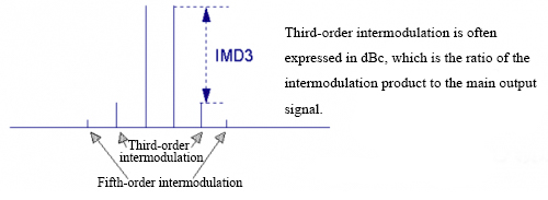
With two monophonic signals separated by ⊿f and of equal level fed into an RF amplifier at the same time, the output spectrum of the amplifier is approximate as follows.
Third-order Cutoff Point
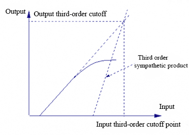
In any microwave unit circuit, the input two-tone signal while increasing by 1dB, the output third-order cross-tone products will increase by 3dB, while the main output signal only increases by 1dB (without considering compression).
Thus the input signal level increases to a certain value, and the output third-order intermodulation products and the main output signal are equal. This point is the third-order cutoff point. The corresponding input signal level is the input third-order cutoff. The corresponding output signal level is the output third-order cutoff point.
Note: The third-order cutoff signal level is impossible to reach. Because at this point the microwave unit circuit has already exceeded its capacity.